Running a Simulation and Plotting

In DMT simulators are interfaced using the abstract classes DutCircuit and DutTcad. These classes define the missing methods which are needed to run any simulator either installed on your pc or on a remote server available using ftp and ssh. The interface uses always the same steps which are shown in the following image:

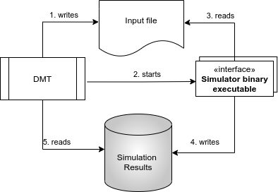
1. A simulation controller SimCon instance calls the make_input method of the dut to simulate. This will then write the input file in a simulation folder. The folder is created in the simulation directory of the Configuration: directories[simulations]/dut_folder/sim_folder. The dut folder name consist of the dut name appended by the unique dut hash. The sim folder consist of the sweep name and the unique sweep hash. This way, no simulation has to be run twice.

2. The simulator binary is called using a sys call with the input file as a parameter in the simulation folder.

3. The simulator reads the input file and executes the simulation accordingly. If it returns a non-zero exit value, the simulation_successful return value is set to False.

4. The simulator writes the simulation results into the simulation folder. This is often done in proprietary binary formats or at least with sorting and naming unknown to DMT.

5. For this the read_result method of the simulated dut is called to read and convert the results into the DMT format. If the simulation binary returned a non-zero exit value, the result is read anyway. Yes we know… but we tested many simulators, and they just behave strange…

After these steps the simulation results are ready to be used. An example code how to make a circuit simulation is shown in the following.

The code for the simulation

import types
import numpy as np
from pathlib import Path
from DMT.core import Sweep, SimCon, Plot, specifiers, DutType, MCard
from DMT.core.circuit import Circuit, CircuitElement, HICUML2_HBT, SHORT, VOLTAGE, RESISTANCE
from DMT.xyce import DutXyce
from DMT.ngspice import DutNgspice

# path to DMT test cases
path_test = Path(__file__).resolve().parent.parent.parent.parent / "test"

# load a hicum/L2 modelcard library by loading the corresponding *va code.
modelcard = MCard(
    ["C", "B", "E", "S", "T"],
    default_module_name="",
    default_subckt_name="",
    va_file=path_test / "test_interface_xyce" / "hicuml2v2p4p0_xyce.va",
)
modelcard.load_model_parameters(
    path_test / "test_core_no_interfaces" / "test_modelcards" / "npn_full.lib",
)
modelcard.update_from_vae(remove_old_parameters=True)


# bind the correct get_circuit method in order to make it easily available for simulation
def get_circuit(self):
    """

    Parameter
    ------------
    modelcard : :class:`~DMT.core.MCard`

    Returns
    -------
    circuit : :class:`~DMT.core.circuit.Circuit`

    """
    circuit_elements = []
    # model instance
    circuit_elements.append(
        CircuitElement(
            "hicumL2_test",
            "Q_H",
            [f"n_{node.upper()}" for node in self.nodes_list],
            parameters=self,
        )
    )

    # BASE NODE CONNECTION #############
    # shorts for current measurement
    circuit_elements.append(CircuitElement(SHORT, "I_B", ["n_B", "n_B_FORCED"]))
    # COLLECTOR NODE CONNECTION #############
    circuit_elements.append(CircuitElement(SHORT, "I_C", ["n_C", "n_C_FORCED"]))
    # EMITTER NODE CONNECTION #############
    circuit_elements.append(CircuitElement(SHORT, "I_E", ["n_E", "0"]))
    # add sources and thermal resistance
    circuit_elements.append(
        CircuitElement(
            VOLTAGE, "V_B", ["n_B_FORCED", "0"], parameters=[("Vdc", "V_B"), ("Vac", "V_B_ac")]
        )
    )
    circuit_elements.append(
        CircuitElement(
            VOLTAGE, "V_C", ["n_C_FORCED", "0"], parameters=[("Vdc", "V_C"), ("Vac", "V_C_ac")]
        )
    )
    circuit_elements += ["V_B=0", "V_C=0", "ac_switch=0", "V_B_ac=1-ac_switch", "V_C_ac=ac_switch"]

    return Circuit(circuit_elements)


modelcard.get_circuit = types.MethodType(get_circuit, modelcard)

duts = []
# init an Xyce Dut
duts.append(DutXyce(None, DutType.npn, modelcard, nodes="C,B,E,S,T", reference_node="E"))
# DMT uses the exact same interface for all circuit simulators, e.g. the call for a ngspice simulation would be:
duts.append(DutNgspice(None, DutType.npn, modelcard, nodes="C,B,E,S,T", reference_node="E"))
# isn't it great?!?

# create a sweep (all DMT Duts can use this!)
# some column names we want to simulate and plot
col_ve = specifiers.VOLTAGE + "E"
col_vb = specifiers.VOLTAGE + "B"
col_vc = specifiers.VOLTAGE + "C"
col_vbe = specifiers.VOLTAGE + ["B", "E"]
col_vcb = specifiers.VOLTAGE + ["C", "B"]
col_vbc = specifiers.VOLTAGE + ["B", "C"]
col_ic = specifiers.CURRENT + "C"
col_freq = specifiers.FREQUENCY
col_ft = specifiers.TRANSIT_FREQUENCY
sweepdef = [
    {"var_name": col_freq, "sweep_order": 4, "sweep_type": "LIST", "value_def": [10e9]},
    {"var_name": col_vb, "sweep_order": 3, "sweep_type": "LIN", "value_def": [0.5, 1, 51]},
    {
        "var_name": col_vc,
        "sweep_order": 3,
        "sweep_type": "SYNC",
        "master": col_vb,
        "offset": col_vcb,
    },
    {"var_name": col_vcb, "sweep_order": 2, "sweep_type": "LIST", "value_def": [-0.5, 0, 0.5]},
    {"var_name": col_ve, "sweep_order": 1, "sweep_type": "CON", "value_def": [0]},
]
outputdef = ["I_C", "I_B"]
othervar = {"TEMP": 300}
sweep = Sweep("gummel", sweepdef=sweepdef, outputdef=outputdef, othervar=othervar)

# The simulation controller can control all simulators implemented in DMT!
sim_con = SimCon()

# Add the desired simulation to the queue and start the simulation
sim_con.append_simulation(dut=duts, sweep=sweep)
sim_con.run_and_read(force=True, remove_simulations=False)

# Plot and save as pdf
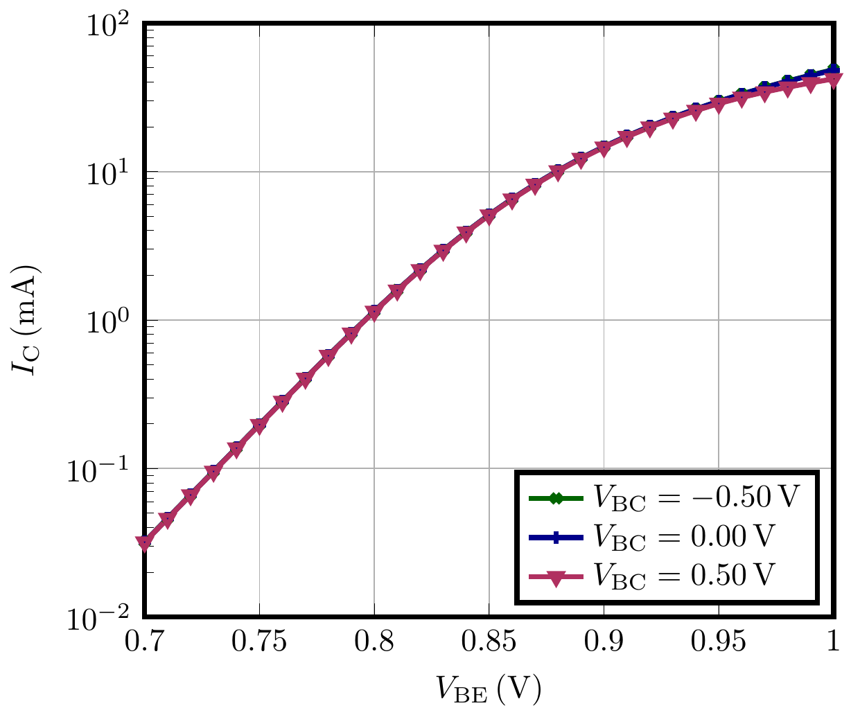
plt_ic = Plot(
    plot_name="J_C(V_BE)",
    x_specifier=col_vbe,
    y_specifier=col_ic,
    y_scale=1e3,
    y_log=True,
    legend_location="lower right",
)
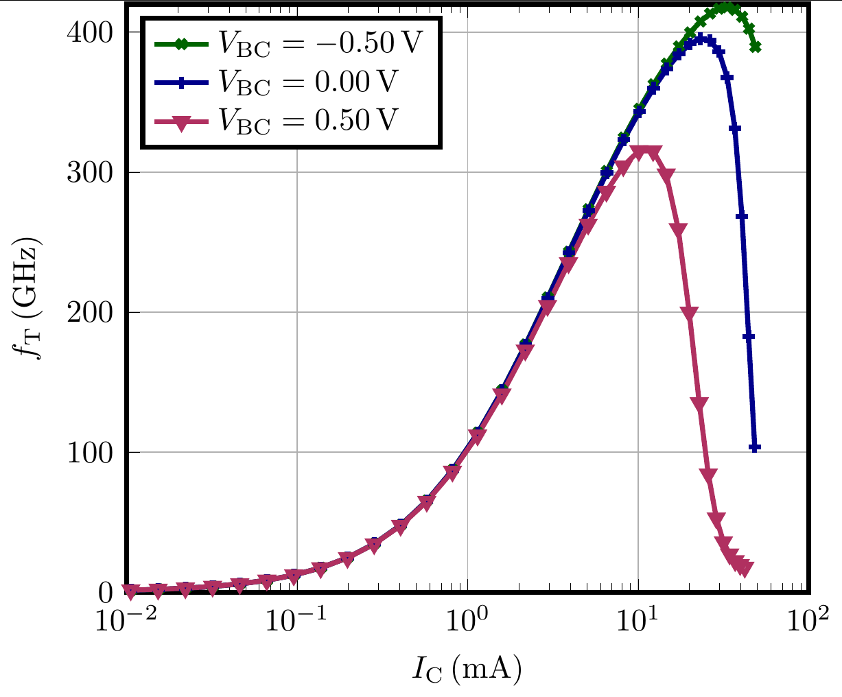
plt_ft = Plot(
    plot_name="F_T(J_C)",
    x_specifier=col_ic,
    x_scale=1e3,
    x_log=True,
    y_specifier=col_ft,
    legend_location="upper left",
)

for dut in duts:
    name = dut.name.split("_")[0] + " "
    # Read back the iv data of the circuit simulator
    data = dut.get_data(sweep=sweep)
    # Ensure derived quantities, e.g. the circuit simulator only gives you S parameters
    data.ensure_specifier_column(col_vbe, ports=["B", "C"])
    data.ensure_specifier_column(col_vbc, ports=["B", "C"])
    data.ensure_specifier_column(col_ft, ports=["B", "C"])

    for i_vbc, vbc, data_vbc in data.iter_unique_col(col_vbc, decimals=3):
        vbc = np.real(vbc)
        plt_ic.add_data_set(
            data_vbc[col_vbe], data_vbc[col_ic], label=name + col_vbc.to_legend_with_value(vbc)
        )
        plt_ft.add_data_set(
            data_vbc[col_ic], data_vbc[col_ft], label=name + col_vbc.to_legend_with_value(vbc)
        )

plt_ic.x_limits = 0.7, 1
plt_ic.y_limits = 1e-2, 1e2
plt_ft.x_limits = 1e-2, 1e2
plt_ft.y_limits = 0, 420

plt_ic.plot_pyqtgraph(show=False)
plt_ft.plot_pyqtgraph()

# plt_ic.save_tikz(
#     Path(__file__).parent.parent / "_static" / "running_a_simulation",
#     standalone=True,
#     build=True,
#     clean=True,
#     width="3in",
# )
# plt_ft.save_tikz(
#     Path(__file__).parent.parent / "_static" / "running_a_simulation",
#     standalone=True,
#     build=True,
#     clean=True,
#     width="3in",
# )

The generated files

J_CV_BE.tex

\documentclass[class=IEEEtran]{standalone}
\usepackage{tikz,amsmath,siunitx}
\usetikzlibrary{arrows,snakes,backgrounds,patterns,matrix,shapes,fit,calc,shadows,plotmarks}
\usepackage[graphics,tightpage,active]{preview}
\usepackage{pgfplots}
\pgfplotsset{compat=newest}
\usetikzlibrary{shapes.geometric}
\PreviewEnvironment{tikzpicture}
\PreviewEnvironment{equation}
\PreviewEnvironment{equation*}
\newlength\figurewidth
\newlength\figureheight
\begin{document}
\setlength\figurewidth{60mm}
\setlength\figureheight{60mm}
\begin{tikzpicture}[font=\normalsize]
\pgfplotsset{every axis/.append style={ultra thick},compat=1.5},
\definecolor{color0}{rgb}{0.00000, 0.39216, 0.00000}
\definecolor{color1}{rgb}{0.00000, 0.00000, 0.54510}
\definecolor{color2}{rgb}{0.69020, 0.18824, 0.37647}

\begin{axis}[scale only axis,ytick pos=left,
width=3in,
xlabel={$V_{\mathrm{BE}}\left(\si{\volt}\right)$},
ylabel={$I_{\mathrm{C}}\left(\si{\milli\ampere}\right)$},
ymode=log,
xmin=0.7,
xmax=1,
restrict x to domain=0.14:5,
log basis x=10,
ymin=0.01,
ymax=100,
restrict y to domain=-10:10,
log basis y=10,
xmajorgrids,
enlargelimits=false,
scaled ticks=false,
ymajorgrids,
x tick style={color=black},
y tick style={color=black},
x grid style={white!69.01960784313725!black},
y grid style={white!69.01960784313725!black},
/tikz/mark repeat=1,
legend style={at={(0.98,0.02)}, anchor=south east,legend cell align=left, align=left},
]
\addplot [color=color0, solid, mark=x, mark options={solid}, mark phase=1, ]
  table[row sep=crcr, x expr=\thisrowno{0}*1.000000e+00, y expr=\thisrowno{1}*1.000000e+03]{
0.5 1.80639e-08\\
0.51 2.63886e-08\\
0.52 3.85387e-08\\
0.53 5.62658e-08\\
0.54 8.21192e-08\\
0.55 1.19808e-07\\
0.56 1.74723e-07\\
0.57 2.54696e-07\\
0.58 3.71093e-07\\
0.59 5.40396e-07\\
0.6 7.8648e-07\\
0.61 1.1439e-06\\
0.62 1.66263e-06\\
0.63 2.41486e-06\\
0.64 3.50476e-06\\
0.65 5.08248e-06\\
0.66 7.36121e-06\\
0.67 1.06546e-05\\
0.68 1.54062e-05\\
0.69 2.22549e-05\\
0.7 3.21173e-05\\
0.71 4.63085e-05\\
0.72 6.67132e-05\\
0.73 9.60261e-05\\
0.74 0.00013808\\
0.75 0.000198284\\
0.76 0.000284178\\
0.77 0.000406103\\
0.78 0.000577911\\
0.79 0.000817588\\
0.8 0.00114752\\
0.81 0.00159412\\
0.82 0.00218643\\
0.83 0.00295385\\
0.84 0.00392323\\
0.85 0.00511616\\
0.86 0.00654728\\
0.87 0.00822382\\
0.88 0.0101462\\
0.89 0.0123096\\
0.9 0.0147051\\
0.91 0.0173211\\
0.92 0.0201448\\
0.93 0.0231623\\
0.94 0.0263597\\
0.95 0.0297231\\
0.96 0.0332389\\
0.97 0.0368942\\
0.98 0.0406763\\
0.99 0.0445729\\
1 0.0485721\\
};
\addlegendentry{$V_{\mathrm{BC}}=\SI{-0.50}{\volt}$}
\addplot [color=color1, solid, mark=+, mark options={solid}, mark phase=1, ]
  table[row sep=crcr, x expr=\thisrowno{0}*1.000000e+00, y expr=\thisrowno{1}*1.000000e+03]{
0.5 1.80136e-08\\
0.51 2.6316e-08\\
0.52 3.8434e-08\\
0.53 5.61146e-08\\
0.54 8.19008e-08\\
0.55 1.19492e-07\\
0.56 1.74267e-07\\
0.57 2.54038e-07\\
0.58 3.70145e-07\\
0.59 5.3903e-07\\
0.6 7.84516e-07\\
0.61 1.14108e-06\\
0.62 1.65858e-06\\
0.63 2.40904e-06\\
0.64 3.49644e-06\\
0.65 5.07059e-06\\
0.66 7.34427e-06\\
0.67 1.06304e-05\\
0.68 1.5372e-05\\
0.69 2.22064e-05\\
0.7 3.20488e-05\\
0.71 4.62117e-05\\
0.72 6.65771e-05\\
0.73 9.58352e-05\\
0.74 0.000137814\\
0.75 0.000197914\\
0.76 0.000283668\\
0.77 0.000405407\\
0.78 0.000576977\\
0.79 0.000816361\\
0.8 0.00114596\\
0.81 0.00159219\\
0.82 0.00218417\\
0.83 0.00295136\\
0.84 0.00392066\\
0.85 0.00511375\\
0.86 0.00654528\\
0.87 0.00822245\\
0.88 0.0101457\\
0.89 0.0123098\\
0.9 0.0147058\\
0.91 0.0173218\\
0.92 0.0201443\\
0.93 0.0231587\\
0.94 0.0263498\\
0.95 0.0297021\\
0.96 0.0331992\\
0.97 0.0368232\\
0.98 0.0405517\\
0.99 0.0443502\\
1 0.0481583\\
};
\addlegendentry{$V_{\mathrm{BC}}=\SI{0.00}{\volt}$}
\addplot [color=color2, solid, mark=triangle, mark options={solid, rotate=180}, mark phase=1, ]
  table[row sep=crcr, x expr=\thisrowno{0}*1.000000e+00, y expr=\thisrowno{1}*1.000000e+03]{
0.5 9.27458e-10\\
0.51 7.4876e-09\\
0.52 1.97108e-08\\
0.53 3.74843e-08\\
0.54 6.33443e-08\\
0.55 1.0098e-07\\
0.56 1.55755e-07\\
0.57 2.35462e-07\\
0.58 3.51408e-07\\
0.59 5.19993e-07\\
0.6 7.64977e-07\\
0.61 1.12075e-06\\
0.62 1.63703e-06\\
0.63 2.38569e-06\\
0.64 3.47042e-06\\
0.65 5.0407e-06\\
0.66 7.30873e-06\\
0.67 1.05868e-05\\
0.68 1.53167e-05\\
0.69 2.21346e-05\\
0.7 3.19532e-05\\
0.71 4.60822e-05\\
0.72 6.63988e-05\\
0.73 9.55863e-05\\
0.74 0.000137462\\
0.75 0.00019741\\
0.76 0.000282939\\
0.77 0.000404337\\
0.78 0.000575387\\
0.79 0.000813969\\
0.8 0.00114233\\
0.81 0.00158668\\
0.82 0.00217581\\
0.83 0.00293882\\
0.84 0.00390223\\
0.85 0.00508728\\
0.86 0.0065082\\
0.87 0.00817167\\
0.88 0.0100772\\
0.89 0.0122182\\
0.9 0.0145821\\
0.91 0.0171503\\
0.92 0.0198959\\
0.93 0.0227786\\
0.94 0.0257388\\
0.95 0.0286968\\
0.96 0.0315715\\
0.97 0.0343251\\
0.98 0.0369758\\
0.99 0.0395621\\
1 0.0421177\\
};
\addlegendentry{$V_{\mathrm{BC}}=\SI{0.50}{\volt}$}
\end{axis}

\end{tikzpicture}
\end{document}

F_TJ_C.tex

\documentclass[class=IEEEtran]{standalone}
\usepackage{tikz,amsmath,siunitx}
\usetikzlibrary{arrows,snakes,backgrounds,patterns,matrix,shapes,fit,calc,shadows,plotmarks}
\usepackage[graphics,tightpage,active]{preview}
\usepackage{pgfplots}
\pgfplotsset{compat=newest}
\usetikzlibrary{shapes.geometric}
\PreviewEnvironment{tikzpicture}
\PreviewEnvironment{equation}
\PreviewEnvironment{equation*}
\newlength\figurewidth
\newlength\figureheight
\begin{document}
\setlength\figurewidth{60mm}
\setlength\figureheight{60mm}
\begin{tikzpicture}[font=\normalsize]
\pgfplotsset{every axis/.append style={ultra thick},compat=1.5},
\definecolor{color0}{rgb}{0.00000, 0.39216, 0.00000}
\definecolor{color1}{rgb}{0.00000, 0.00000, 0.54510}
\definecolor{color2}{rgb}{0.69020, 0.18824, 0.37647}

\begin{axis}[scale only axis,ytick pos=left,
width=3in,
xlabel={$I_{\mathrm{C}}\left(\si{\milli\ampere}\right)$},
ylabel={$f_{\mathrm{T}}\left(\si{\giga\hertz}\right)$},
xmode=log,
xmin=0.01,
xmax=100,
restrict x to domain=-10:10,
log basis x=10,
ymin=0,
ymax=420,
restrict y to domain=0:2100,
log basis y=10,
xmajorgrids,
enlargelimits=false,
scaled ticks=false,
ymajorgrids,
x tick style={color=black},
y tick style={color=black},
x grid style={white!69.01960784313725!black},
y grid style={white!69.01960784313725!black},
/tikz/mark repeat=1,
legend style={at={(0.02,0.98)}, anchor=north west,legend cell align=left, align=left},
]
\addplot [color=color0, solid, mark=x, mark options={solid}, mark phase=1, ]
  table[row sep=crcr, x expr=\thisrowno{0}*1.000000e+03, y expr=\thisrowno{1}*1.000000e-09]{
1.80639e-08 9.26724e+10\\
2.63886e-08 6.116e+10\\
3.85387e-08 4.07307e+10\\
5.62658e-08 2.72951e+10\\
8.21192e-08 1.83731e+10\\
1.19808e-07 1.24098e+10\\
1.74723e-07 8.40734e+09\\
2.54696e-07 5.71522e+09\\
3.71093e-07 3.90476e+09\\
5.40396e-07 2.69183e+09\\
7.8648e-07 1.88791e+09\\
1.1439e-06 1.36868e+09\\
1.66263e-06 1.05367e+09\\
2.41486e-06 8.93344e+08\\
3.50476e-06 8.6136e+08\\
5.08248e-06 9.50402e+08\\
7.36121e-06 1.16982e+09\\
1.06546e-05 1.54797e+09\\
1.54062e-05 2.13321e+09\\
2.22549e-05 3.00092e+09\\
3.21173e-05 4.26251e+09\\
4.63085e-05 6.07866e+09\\
6.67132e-05 8.67614e+09\\
9.60261e-05 1.23675e+10\\
0.00013808 1.75706e+10\\
0.000198284 2.48224e+10\\
0.000284178 3.47723e+10\\
0.000406103 4.81356e+10\\
0.000577911 6.55815e+10\\
0.000817588 8.7547e+10\\
0.00114752 1.14004e+11\\
0.00159412 1.44281e+11\\
0.00218643 1.77057e+11\\
0.00295385 2.10612e+11\\
0.00392323 2.43229e+11\\
0.00511616 2.73564e+11\\
0.00654728 3.00814e+11\\
0.00822382 3.24687e+11\\
0.0101462 3.45246e+11\\
0.0123096 3.62742e+11\\
0.0147051 3.77484e+11\\
0.0173211 3.8975e+11\\
0.0201448 3.99749e+11\\
0.0231623 4.07587e+11\\
0.0263597 4.1327e+11\\
0.0297231 4.16694e+11\\
0.0332389 4.17661e+11\\
0.0368942 4.15882e+11\\
0.0406763 4.10984e+11\\
0.0445729 4.02459e+11\\
0.0485721 3.89436e+11\\
};
\addlegendentry{$V_{\mathrm{BC}}=\SI{-0.50}{\volt}$}
\addplot [color=color1, solid, mark=+, mark options={solid}, mark phase=1, ]
  table[row sep=crcr, x expr=\thisrowno{0}*1.000000e+03, y expr=\thisrowno{1}*1.000000e-09]{
1.80136e-08 1.18811e+11\\
2.6316e-08 7.83898e+10\\
3.8434e-08 5.2163e+10\\
5.61146e-08 3.49168e+10\\
8.19008e-08 2.3472e+10\\
1.19492e-07 1.58298e+10\\
1.74267e-07 1.07058e+10\\
2.54038e-07 7.26219e+09\\
3.70145e-07 4.94724e+09\\
5.3903e-07 3.39509e+09\\
7.84516e-07 2.36284e+09\\
1.14108e-06 1.68982e+09\\
1.65858e-06 1.27113e+09\\
2.40904e-06 1.04075e+09\\
3.49644e-06 9.61219e+08\\
5.07059e-06 1.01778e+09\\
7.34427e-06 1.21485e+09\\
1.06304e-05 1.57731e+09\\
1.5372e-05 2.15124e+09\\
2.22064e-05 3.01038e+09\\
3.20488e-05 4.26494e+09\\
4.62117e-05 6.0746e+09\\
6.65771e-05 8.6653e+09\\
9.58352e-05 1.23487e+10\\
0.000137814 1.75416e+10\\
0.000197914 2.47799e+10\\
0.000283668 3.47112e+10\\
0.000405407 4.80487e+10\\
0.000576977 6.54589e+10\\
0.000816361 8.73747e+10\\
0.00114596 1.13764e+11\\
0.00159219 1.4395e+11\\
0.00218417 1.76607e+11\\
0.00295136 2.10013e+11\\
0.00392066 2.4245e+11\\
0.00511375 2.72568e+11\\
0.00654528 2.99559e+11\\
0.00822245 3.23104e+11\\
0.0101457 3.43216e+11\\
0.0123098 3.60052e+11\\
0.0147058 3.73758e+11\\
0.0173218 3.84361e+11\\
0.0201443 3.91677e+11\\
0.0231587 3.95214e+11\\
0.0263498 3.93989e+11\\
0.0297021 3.8609e+11\\
0.0331992 3.67653e+11\\
0.0368232 3.31384e+11\\
0.0405517 2.68355e+11\\
0.0443502 1.82719e+11\\
0.0481583 1.03973e+11\\
};
\addlegendentry{$V_{\mathrm{BC}}=\SI{0.00}{\volt}$}
\addplot [color=color2, solid, mark=triangle, mark options={solid, rotate=180}, mark phase=1, ]
  table[row sep=crcr, x expr=\thisrowno{0}*1.000000e+03, y expr=\thisrowno{1}*1.000000e-09]{
9.27458e-10 1.64549e+11\\
7.4876e-09 1.0934e+11\\
1.97108e-08 7.30099e+10\\
3.74843e-08 4.89271e+10\\
6.33443e-08 3.28787e+10\\
1.0098e-07 2.21443e+10\\
1.55755e-07 1.49455e+10\\
2.35462e-07 1.01101e+10\\
3.51408e-07 6.8613e+09\\
5.19993e-07 4.68234e+09\\
7.64977e-07 3.22929e+09\\
1.12075e-06 2.27372e+09\\
1.63703e-06 1.66525e+09\\
2.38569e-06 1.30716e+09\\
3.47042e-06 1.14137e+09\\
5.0407e-06 1.13935e+09\\
7.30873e-06 1.29639e+09\\
1.05868e-05 1.63104e+09\\
1.53167e-05 2.18521e+09\\
2.21346e-05 3.02958e+09\\
3.19532e-05 4.27201e+09\\
4.60822e-05 6.07009e+09\\
6.63988e-05 8.6474e+09\\
9.55863e-05 1.23123e+10\\
0.000137462 1.74764e+10\\
0.00019741 2.46663e+10\\
0.000282939 3.45144e+10\\
0.000404337 4.77081e+10\\
0.000575387 6.48747e+10\\
0.000813969 8.63927e+10\\
0.00114233 1.12165e+11\\
0.00158668 1.41452e+11\\
0.00217581 1.72884e+11\\
0.00293882 2.04708e+11\\
0.00390223 2.35161e+11\\
0.00508728 2.62745e+11\\
0.0065082 2.86241e+11\\
0.00817167 3.04381e+11\\
0.0100772 3.15206e+11\\
0.0122182 3.15161e+11\\
0.0145821 2.98536e+11\\
0.0171503 2.59523e+11\\
0.0198959 1.99872e+11\\
0.0227786 1.35295e+11\\
0.0257388 8.44329e+10\\
0.0286968 5.29578e+10\\
0.0315715 3.59953e+10\\
0.0343251 2.72259e+10\\
0.0369758 2.24818e+10\\
0.0395621 1.96668e+10\\
0.0421177 1.78143e+10\\
};
\addlegendentry{$V_{\mathrm{BC}}=\SI{0.50}{\volt}$}
\end{axis}

\end{tikzpicture}
\end{document}