Basic data handling example

The example code

"""
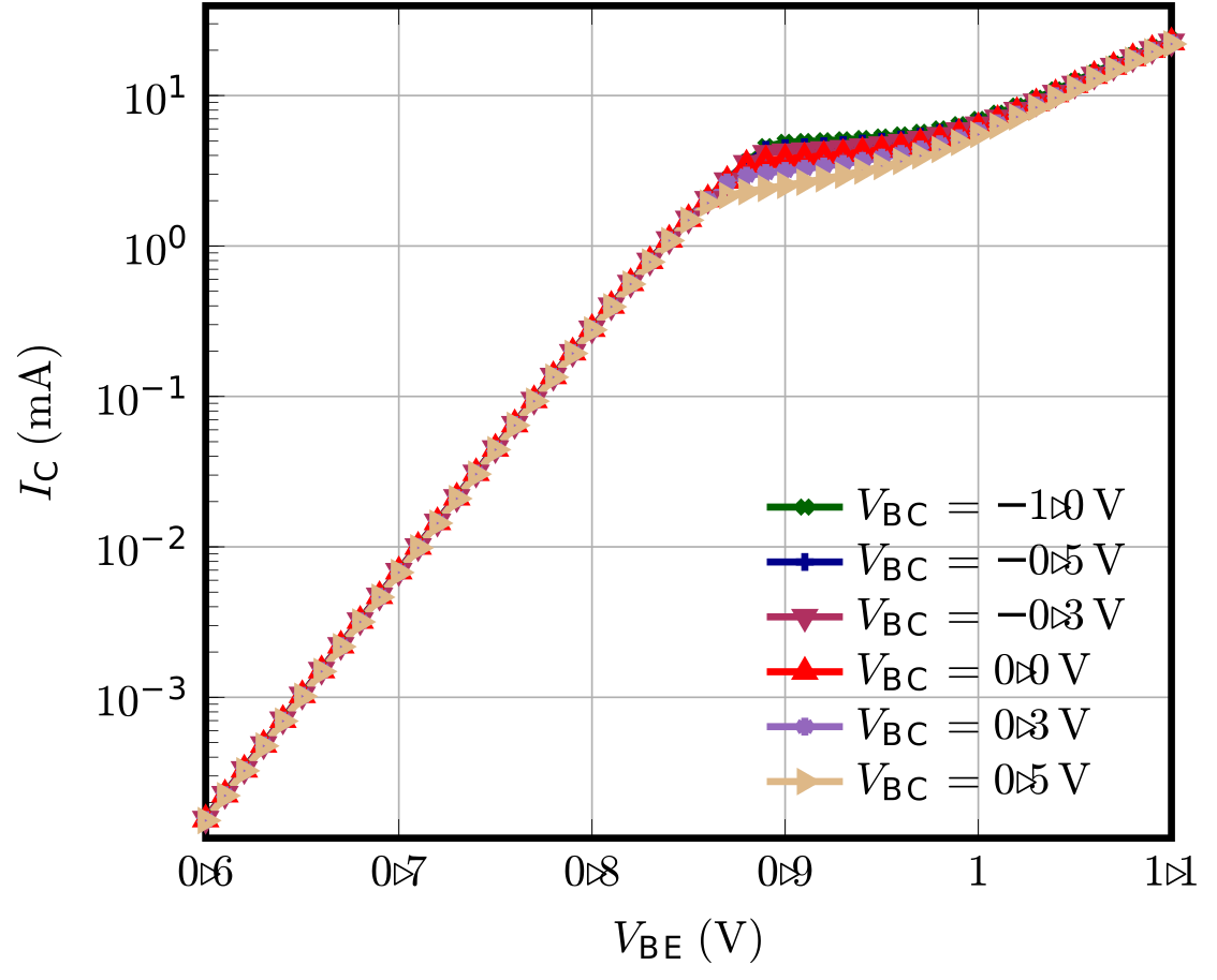
This example shows the basic data handling with python.
We will read data, clean it, calculate with the data and then plot.
"""
from pathlib import Path
from DMT.core import read_data, specifiers, Plot

# path to static folder:
path_static = Path(__file__).resolve().parent.parent / "_static"

# some specifiers, they allow consistent access to electrical data
# all interfaces of DMT adhere to these specifiers!
col_vbe = specifiers.VOLTAGE + ["B", "E"]
col_vbc = specifiers.VOLTAGE + ["B", "C"]
col_ic = specifiers.CURRENT + "C"
col_ib = specifiers.CURRENT + "B"

# read data using the given method
data = read_data(path_static / "HBT_vbc.elpa")

# "clean" the data so we have DMT-specifier in it.
# This ensure that the read-in data is consistent with the DMT specifiers.
# clean data additionally removes all voltages and only potentials remain
data = data.clean_data(["B", "C", "E"], reference_node="E")
# adjust unit from read in file (currents were in mA, DMT uses always basic units):
data[col_ic] = data[col_ic] * 1e-3
data[col_ib] = data[col_ib] * 1e-3
# The "ensure_specifier_column" method can be used to ensure that a given derived
# electrical quantity, such as a voltage, is inside the dataframe. If it is not there,
# an algorithm will try to generate the quantity.
data.ensure_specifier_column(col_vbe)
data.ensure_specifier_column(col_vbc)

# generate the plot object with proper axis and legend location
plot = Plot(
    "I_C(V_BE)",
    x_specifier=col_vbe,
    y_specifier=col_ic,
    y_scale=1e3,
    y_log=True,
    legend_location="lower right",
)
plot.legend_frame = False
plot.x_limits = (0.6, 1.1)

# fill the gummel plot with a line for each V_BC
for _index, vbc, data_vbc in data.iter_unique_col(col_vbc, decimals=3):
    plot.add_data_set(
        data_vbc[col_vbe],
        data_vbc[col_ic],
        label="${:s}= \\SI{{{:.1f}}}{{\\volt}}$".format(col_vbc.to_tex(), vbc),
    )

# show the plot (DMT has three plotting back-ends: matplotlib, pyqtgraph and tikz)
# plot.plot_pyqtgraph()
plot.plot_py()
# save the plot as tikz and build it
plot.save_tikz(
    path_static,
    standalone=True,
    build=True,
    clean=True,
    width="3in",
)

The generated files

I_CV_BE.pdf

I_CV_BE.tex

\documentclass[class=IEEEtran]{standalone}
\usepackage{tikz,amsmath,siunitx}
\usetikzlibrary{arrows,snakes,backgrounds,patterns,matrix,shapes,fit,calc,shadows,plotmarks}
\usepackage[graphics,tightpage,active]{preview}
\usepackage{pgfplots}
\pgfplotsset{compat=newest}
\usetikzlibrary{shapes.geometric}
\PreviewEnvironment{tikzpicture}
\PreviewEnvironment{equation}
\PreviewEnvironment{equation*}
\newlength\figurewidth
\newlength\figureheight
\begin{document}
\setlength\figurewidth{60mm}
\setlength\figureheight{60mm}
\begin{tikzpicture}[font=\normalsize]
\pgfplotsset{every axis/.append style={ultra thick},compat=1.5},
\definecolor{color0}{rgb}{0.00000, 0.39216, 0.00000}
\definecolor{color1}{rgb}{0.00000, 0.00000, 0.54510}
\definecolor{color2}{rgb}{0.69020, 0.18824, 0.37647}
\definecolor{color3}{rgb}{1.00000, 0.00000, 0.00000}
\definecolor{color4}{rgb}{0.58039, 0.40392, 0.74118}
\definecolor{color5}{rgb}{0.87059, 0.72157, 0.52941}

\begin{axis}[scale only axis,ytick pos=left,
width=3in,
xlabel={$V_{\mathrm{BE}}\left(\si{\volt}\right)$},
ylabel={$I_{\mathrm{C}}\left(\si{\milli\ampere}\right)$},
ymode=log,
xmin=0.6,
xmax=1.1,
restrict x to domain=0.12:5.5,
log basis x=10,
ymin=0.000115874,
ymax=39.5057,
restrict y to domain=-19.6801:7.9833,
log basis y=10,
xmajorgrids,
enlargelimits=false,
scaled ticks=true,
ymajorgrids,
x tick style={color=black},
y tick style={color=black},
x grid style={white!69.01960784313725!black},
y grid style={white!69.01960784313725!black},
/tikz/mark repeat=1,
legend style={at={(0.98,0.02)}, anchor=south east,legend cell align=left, align=left, fill=none, draw=none},
]
\addplot [color=color0, solid, mark=x, mark options={solid}, mark phase=1, ]
  table[row sep=crcr, x expr=\thisrowno{0}*1.000000e+00, y expr=\thisrowno{1}*1.000000e+03]{
0.6 1.57931e-07\\
0.61 2.31036e-07\\
0.62 3.37917e-07\\
0.63 4.94143e-07\\
0.64 7.22433e-07\\
0.65 1.05593e-06\\
0.66 1.54295e-06\\
0.67 2.25389e-06\\
0.68 3.29124e-06\\
0.69 4.80404e-06\\
0.7 7.00881e-06\\
0.71 1.02196e-05\\
0.72 1.4891e-05\\
0.73 2.16796e-05\\
0.74 3.15304e-05\\
0.75 4.57977e-05\\
0.76 6.64121e-05\\
0.77 9.61046e-05\\
0.78 0.000138701\\
0.79 0.00019949\\
0.8 0.000285662\\
0.81 0.000406776\\
0.82 0.000575186\\
0.83 0.000806309\\
0.84 0.00111858\\
0.85 0.00153297\\
0.86 0.00207183\\
0.87 0.002757\\
0.88 0.00360467\\
0.89 0.0045765\\
0.9 0.00488923\\
0.91 0.00494777\\
0.92 0.0050081\\
0.93 0.00508284\\
0.94 0.00517917\\
0.95 0.00530589\\
0.96 0.00547472\\
0.97 0.00569853\\
0.98 0.00599919\\
0.99 0.00640369\\
1 0.00694022\\
1.01 0.00763601\\
1.02 0.00851569\\
1.03 0.00959848\\
1.04 0.0109032\\
1.05 0.0124441\\
1.06 0.0142227\\
1.07 0.016231\\
1.08 0.0184492\\
1.09 0.0208371\\
1.1 0.023341\\
};
\addlegendentry{$V_{\mathrm{BC}}= \SI{-1.0}{\volt}$}
\addplot [color=color1, solid, mark=+, mark options={solid}, mark phase=1, ]
  table[row sep=crcr, x expr=\thisrowno{0}*1.000000e+00, y expr=\thisrowno{1}*1.000000e+03]{
0.6 1.56378e-07\\
0.61 2.28783e-07\\
0.62 3.34651e-07\\
0.63 4.8941e-07\\
0.64 7.15578e-07\\
0.65 1.04601e-06\\
0.66 1.5286e-06\\
0.67 2.23314e-06\\
0.68 3.26127e-06\\
0.69 4.76079e-06\\
0.7 6.94645e-06\\
0.71 1.01298e-05\\
0.72 1.47619e-05\\
0.73 2.14943e-05\\
0.74 3.1265e-05\\
0.75 4.54186e-05\\
0.76 6.58721e-05\\
0.77 9.53386e-05\\
0.78 0.000137619\\
0.79 0.000197973\\
0.8 0.000283549\\
0.81 0.000403858\\
0.82 0.0005712\\
0.83 0.000800931\\
0.84 0.00111142\\
0.85 0.00152352\\
0.86 0.00205942\\
0.87 0.00274027\\
0.88 0.00357795\\
0.89 0.00435599\\
0.9 0.00447169\\
0.91 0.00453578\\
0.92 0.00460511\\
0.93 0.00468889\\
0.94 0.00479386\\
0.95 0.00492834\\
0.96 0.00510194\\
0.97 0.00532997\\
0.98 0.00563537\\
0.99 0.00604573\\
1 0.00659001\\
1.01 0.00729441\\
1.02 0.00818138\\
1.03 0.00927128\\
1.04 0.0105796\\
1.05 0.0121198\\
1.06 0.0138983\\
1.07 0.0159047\\
1.08 0.0181156\\
1.09 0.0204957\\
1.1 0.0229951\\
};
\addlegendentry{$V_{\mathrm{BC}}= \SI{-0.5}{\volt}$}
\addplot [color=color2, solid, mark=triangle, mark options={solid, rotate=180}, mark phase=1, ]
  table[row sep=crcr, x expr=\thisrowno{0}*1.000000e+00, y expr=\thisrowno{1}*1.000000e+03]{
0.6 1.55669e-07\\
0.61 2.27755e-07\\
0.62 3.3316e-07\\
0.63 4.8725e-07\\
0.64 7.12449e-07\\
0.65 1.04148e-06\\
0.66 1.52204e-06\\
0.67 2.22367e-06\\
0.68 3.24757e-06\\
0.69 4.74102e-06\\
0.7 6.91795e-06\\
0.71 1.00888e-05\\
0.72 1.47029e-05\\
0.73 2.14096e-05\\
0.74 3.11435e-05\\
0.75 4.52449e-05\\
0.76 6.56247e-05\\
0.77 9.49873e-05\\
0.78 0.000137123\\
0.79 0.000197275\\
0.8 0.000282575\\
0.81 0.00040251\\
0.82 0.000569351\\
0.83 0.000798421\\
0.84 0.00110804\\
0.85 0.001519\\
0.86 0.00205332\\
0.87 0.00273153\\
0.88 0.00355995\\
0.89 0.00415437\\
0.9 0.0042477\\
0.91 0.00431721\\
0.92 0.00439326\\
0.93 0.00448412\\
0.94 0.00459637\\
0.95 0.00473761\\
0.96 0.00491714\\
0.97 0.00515087\\
0.98 0.00546182\\
0.99 0.00587797\\
1 0.00642824\\
1.01 0.00713864\\
1.02 0.0080306\\
1.03 0.00912394\\
1.04 0.010435\\
1.05 0.0119757\\
1.06 0.0137532\\
1.07 0.0157592\\
1.08 0.0179685\\
1.09 0.0203448\\
1.1 0.0228409\\
};
\addlegendentry{$V_{\mathrm{BC}}= \SI{-0.3}{\volt}$}
\addplot [color=color3, solid, mark=triangle, mark options={solid, rotate=0}, mark phase=1, ]
  table[row sep=crcr, x expr=\thisrowno{0}*1.000000e+00, y expr=\thisrowno{1}*1.000000e+03]{
0.6 1.54461e-07\\
0.61 2.26002e-07\\
0.62 3.30619e-07\\
0.63 4.83566e-07\\
0.64 7.07112e-07\\
0.65 1.03375e-06\\
0.66 1.51086e-06\\
0.67 2.20749e-06\\
0.68 3.2242e-06\\
0.69 4.70728e-06\\
0.7 6.86928e-06\\
0.71 1.00186e-05\\
0.72 1.4602e-05\\
0.73 2.12647e-05\\
0.74 3.09358e-05\\
0.75 4.49479e-05\\
0.76 6.52011e-05\\
0.77 9.43853e-05\\
0.78 0.000136271\\
0.79 0.000196076\\
0.8 0.000280897\\
0.81 0.00040018\\
0.82 0.00056614\\
0.83 0.000794028\\
0.84 0.00110206\\
0.85 0.00151084\\
0.86 0.00204185\\
0.87 0.00271311\\
0.88 0.0034726\\
0.89 0.00371751\\
0.9 0.00380651\\
0.91 0.00388909\\
0.92 0.00398065\\
0.93 0.00408838\\
0.94 0.00421844\\
0.95 0.00437727\\
0.96 0.0045744\\
0.97 0.00482538\\
0.98 0.00515277\\
0.99 0.0055848\\
1 0.00615026\\
1.01 0.00687402\\
1.02 0.00777703\\
1.03 0.00887756\\
1.04 0.0101932\\
1.05 0.0117365\\
1.06 0.0135125\\
1.07 0.0155162\\
1.08 0.0177239\\
1.09 0.0200962\\
1.1 0.0225853\\
};
\addlegendentry{$V_{\mathrm{BC}}= \SI{0.0}{\volt}$}
\addplot [color=color4, solid, mark=asterisk, mark options={solid}, mark phase=1, ]
  table[row sep=crcr, x expr=\thisrowno{0}*1.000000e+00, y expr=\thisrowno{1}*1.000000e+03]{
0.6 1.52964e-07\\
0.61 2.2383e-07\\
0.62 3.27468e-07\\
0.63 4.78998e-07\\
0.64 7.00492e-07\\
0.65 1.02416e-06\\
0.66 1.49698e-06\\
0.67 2.18742e-06\\
0.68 3.19518e-06\\
0.69 4.66537e-06\\
0.7 6.80881e-06\\
0.71 9.93149e-06\\
0.72 1.44766e-05\\
0.73 2.10844e-05\\
0.74 3.06771e-05\\
0.75 4.45776e-05\\
0.76 6.46723e-05\\
0.77 9.36325e-05\\
0.78 0.000135203\\
0.79 0.000194567\\
0.8 0.000278776\\
0.81 0.000397211\\
0.82 0.000562003\\
0.83 0.000788269\\
0.84 0.00109399\\
0.85 0.00149917\\
0.86 0.00202287\\
0.87 0.00264508\\
0.88 0.00293828\\
0.89 0.00305683\\
0.9 0.00315725\\
0.91 0.00326133\\
0.92 0.00337801\\
0.93 0.00351352\\
0.94 0.00367362\\
0.95 0.00386512\\
0.96 0.00409744\\
0.97 0.00438453\\
0.98 0.00474703\\
0.99 0.0052115\\
1 0.00580521\\
1.01 0.00655175\\
1.02 0.00747146\\
1.03 0.00858347\\
1.04 0.00990534\\
1.05 0.0114516\\
1.06 0.0132283\\
1.07 0.0152289\\
1.08 0.0174323\\
1.09 0.0198004\\
1.1 0.0222831\\
};
\addlegendentry{$V_{\mathrm{BC}}= \SI{0.3}{\volt}$}
\addplot [color=color5, solid, mark=triangle, mark options={solid, rotate=270}, mark phase=1, ]
  table[row sep=crcr, x expr=\thisrowno{0}*1.000000e+00, y expr=\thisrowno{1}*1.000000e+03]{
0.6 1.51634e-07\\
0.61 2.21907e-07\\
0.62 3.24685e-07\\
0.63 4.74968e-07\\
0.64 6.94657e-07\\
0.65 1.01571e-06\\
0.66 1.48476e-06\\
0.67 2.16974e-06\\
0.68 3.16963e-06\\
0.69 4.62845e-06\\
0.7 6.75553e-06\\
0.71 9.85468e-06\\
0.72 1.4366e-05\\
0.73 2.09253e-05\\
0.74 3.04486e-05\\
0.75 4.425e-05\\
0.76 6.42035e-05\\
0.77 9.2963e-05\\
0.78 0.000134249\\
0.79 0.000193211\\
0.8 0.00027685\\
0.81 0.000394476\\
0.82 0.0005581\\
0.83 0.000782617\\
0.84 0.00108542\\
0.85 0.00148359\\
0.86 0.00193031\\
0.87 0.00216209\\
0.88 0.00229712\\
0.89 0.00241257\\
0.9 0.00252828\\
0.91 0.0026535\\
0.92 0.00279469\\
0.93 0.00295766\\
0.94 0.00314863\\
0.95 0.00337497\\
0.96 0.00364612\\
0.97 0.003975\\
0.98 0.00437957\\
0.99 0.00488256\\
1 0.00550803\\
1.01 0.00627846\\
1.02 0.00721484\\
1.03 0.00833756\\
1.04 0.00966576\\
1.05 0.0112146\\
1.06 0.0129913\\
1.07 0.0149899\\
1.08 0.0171885\\
1.09 0.01955\\
1.1 0.0220256\\
};
\addlegendentry{$V_{\mathrm{BC}}= \SI{0.5}{\volt}$}
\end{axis}

\end{tikzpicture}
\end{document}